How to Create Stunning Scatter Plots using Python Matplotlib

Scatter plots are arguably the most powerful tool in a data scientist's arsenal. They don't just show data points; they tell stories about relationships, correlations, and clusters that might otherwise go unnoticed.

While there are many libraries out there, Matplotlib remains the grandfather of Python plotting – powerful, flexible, and essential to master. But let's be honest: the default Matplotlib styles can look a bit... 1990s.

In this guide, I'll walk you through how to create a scatter plot that not only displays your data accurately but looks professional and presentation-ready.

Prerequisites

Before we dive in, make sure you have Python installed and the necessary libraries. If you haven't already, fire up your terminal:


python
pip install matplotlib numpy pandas

We'll use numpy to generate some sample data for this tutorial.

Step 1: The Basic Scatter Plot

Let's start with the absolute basics. Here is the "Hello World" of scatter plots.


python
import matplotlib.pyplot as plt
import numpy as np

# Generate random data
x = np.random.rand(50)
y = np.random.rand(50)

plt.scatter(x, y)
plt.show()

This works, but it's plain. It gets the job done for quick data exploration, but you wouldn't want to put this in a client report or a publication.

Step 2: Adding Meaning with Color and Size

A scatter plot becomes truly powerful when you encode more dimensions into it. You're not limited to just X and Y coordinates; you can use color and size to represent third and fourth variables.

Let's say we want to visualize the correlation between Ad Spend (X) and Sales (Y), where the size of the bubble represents Market Size, and the color represents Profitability.


python
# Enhanced data
colors = np.random.rand(50)
sizes = 1000 * np.random.rand(50)

plt.scatter(x, y, c=colors, s=sizes, alpha=0.5, cmap='viridis')
plt.colorbar(label='Profitability Scale')  # Show the color scale
plt.show()

We added alpha=0.5 to make the points semi-transparent. This is a pro tip: it helps you see where points overlap (density) and prevents the plot from looking like a solid blob of color.

Step 3: Making It Beautiful (UI/UX)

The user asked for a "good UI," and in the context of data viz, that means readability and aesthetics. Let's ditch the default style and customize the chart to look modern.

Matplotlib has built-in styles, but manually tweaking the grid and fonts gives the best results.


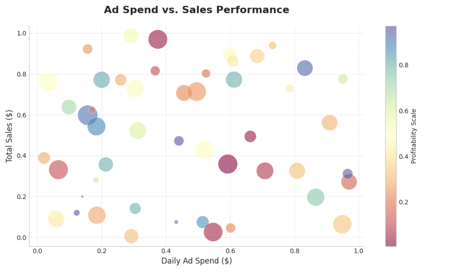
python
# Set a clean style
plt.style.use('seaborn-v0_8-whitegrid')

plt.figure(figsize=(10, 6))

# Customizing the plot
plt.scatter(x, y, 
            c=colors, 
            s=sizes, 
            alpha=0.6, 
            cmap='Spectral', 
            edgecolors='w',  # White edge makes points pop
            linewidth=0.5)

# Adding labels with better fonts
plt.title('Ad Spend vs. Sales Performance', fontsize=16, fontweight='bold', pad=20)
plt.xlabel('Daily Ad Spend ($)', fontsize=12)
plt.ylabel('Total Sales ($)', fontsize=12)

# Customizing the grid
plt.grid(True, linestyle='--', alpha=0.7)

# Remove top and right spines for a cleaner look
plt.gca().spines['top'].set_visible(False)
plt.gca().spines['right'].set_visible(False)

plt.show()

Conclusion

Creating a scatter plot in Python is easy, but creating a great one takes a bit of extra care. By adjusting transparencies, choosing the right colormaps, and cleaning up the chart junk (like unnecessary spines), you can turn a simple plot into a compelling data story.

Final Complete Code

Here is the complete snippet you can copy and run to generate the beautiful scatter plot we built today.


python
import matplotlib.pyplot as plt
import numpy as np

# 1. Setup the data
np.random.seed(42) # for reproducibility
x = np.random.rand(50)
y = np.random.rand(50)
colors = np.random.rand(50)
sizes = 1000 * np.random.rand(50)

# 2. Set the style
# Note: Styles may vary by matplotlib version. 
# Check plt.style.available for options on your system.
plt.style.use('seaborn-v0_8-whitegrid')

# 3. Create the figure
plt.figure(figsize=(10, 6))

# 4. Plot the data
scatter = plt.scatter(x, y, 
            c=colors, 
            s=sizes, 
            alpha=0.6, 
            cmap='Spectral', 
            edgecolors='w', 
            linewidth=0.5)

# 5. Add specific aesthetics
plt.colorbar(scatter, label='Profitability Scale')
plt.title('Ad Spend vs. Sales Performance', fontsize=16, fontweight='bold', pad=20)
plt.xlabel('Daily Ad Spend ($)', fontsize=12)
plt.ylabel('Total Sales ($)', fontsize=12)

# 6. Refine the grid and axes
plt.grid(True, linestyle='--', alpha=0.5)
plt.gca().spines['top'].set_visible(False)
plt.gca().spines['right'].set_visible(False)

# 7. Show result
plt.show()

Final Scatter Plot Output

Remember, the goal of any visualization is clarity. Only add complexity (like color or size variations) if it adds information. Happy coding!

Scatter Plot Maker