How to Calculate Standard Deviation Step by Step (With Worked Examples)

A few years ago a friend of mine, a high school maths teacher, showed me two report cards from two different classes she had been teaching. Both classes had the same average score on the same test: 72 out of 100. By every official number the school cared about, the classes looked identical.

Then she showed me the actual scores. One class had everyone hovering between 68 and 76. The other class had a few students at 35 and a few at 98. Same average. Two completely different stories.

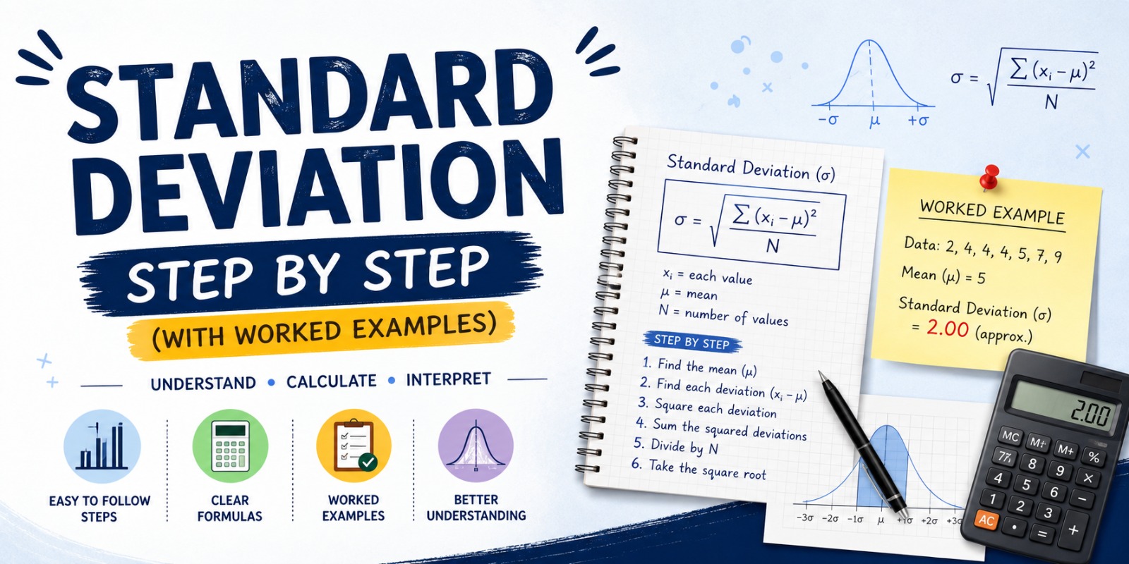
Standard deviation is the number that finally tells those two stories apart. It is one of the most useful ideas in statistics, and it is also one of the most over-complicated. So let us calculate it from scratch, with real numbers, and without any hand-waving.

Why averages lie about your data

The mean (or average) is a single point. It tells you where the middle of your data sits. What it does not tell you is whether your numbers are bunched tightly around that middle or scattered all over the place.

Picture two coffee shops. Both claim an average wait time of 5 minutes. At the first shop, every customer waits somewhere between 4 and 6 minutes. At the second, half the customers wait 1 minute and the other half wait 9. The signs at the door would say the same thing, but your experience as a customer would not be remotely the same.

“The mean tells you where the centre is. Standard deviation tells you how seriously to trust the centre.”

What standard deviation actually measures

Standard deviation answers a single question: on average, how far is a typical data point from the mean?

That is it. Strip away the Greek letters and the symbols, and the formula is just measuring distance. The complications are mostly bookkeeping: we square the distances to keep them positive, we average the squares, and we take a square root at the end to undo the squaring. Every step has a reason.

See the spread for yourself

Before any maths, get a feel for what we are measuring. Both datasets below have the same mean. The only thing that changes is how tightly the dots cluster around it.

Interactive

mean = 50.0

100

Both datasets have the same mean (50). Toggle to feel the spread that standard deviation actually measures.

The low-spread dataset has a standard deviation around 2. The high-spread one is closer to 22. Same average, eleven times more scatter. If a manager only looked at the average, those two situations would look the same. If they looked at the standard deviation, they would treat them very differently.

Population vs sample: the n vs n−1 trap

Before we touch a single number, we need to settle one decision that trips up almost everyone. There are two flavours of standard deviation, and they differ in one tiny place.

If you have data for every single item you care about (every employee in your company, every test paper in this exact class, every product made today), you have a population. You divide by $N$ .

If your data is a sample drawn from some larger population (a survey of 200 people meant to represent a city, a batch of products meant to represent a factory), you divide by $n - 1$ instead.

Population SD

\sigma = \sqrt{\dfrac{\sum (x_i - \mu)^2}{N}}

Use when you have every value in the group you care about.

Sample SD

s = \sqrt{\dfrac{\sum (x_i - \bar{x})^2}{n - 1}}

Use when your data is a sample from a larger group.

Rule of thumb: if you are not sure which one you have, you almost certainly have a sample. Real-world data is rarely complete. Use $n - 1$ .

The five steps, in plain English

Every standard deviation calculation is the same five steps, in the same order. Once you have done it twice, it becomes muscle memory.

Find the mean

Add up all your values and divide by how many there are. This is your reference point.

Subtract the mean from each value

The result is called a deviation. Some will be positive, some negative. That is fine.

Square every deviation

Squaring kills the negative signs and exaggerates large differences, which is what we want.

Average the squared deviations

Divide by

N

for a population or

n - 1

for a sample. The result is the variance.

Take the square root

This undoes the squaring from step 3 and brings the answer back to your original units. That final number is the standard deviation.

Worked example 1: population SD

Let us calculate the standard deviation of five test scores. Imagine these are the scores of every student in a small study group, so this is the entire group we care about. That makes it a population.

Scores: 80, 82, 78, 85, 75

Step 1: Find the mean

\mu = \dfrac{80 + 82 + 78 + 85 + 75}{5} = \dfrac{400}{5} = 80

The mean is 80. Now we measure how far each score sits from 80.

Step 2 to 4: Build a table

Doing this in a table is the single biggest thing that stops you making errors. Three columns: the value, its deviation from the mean, and the squared deviation.

Population SD worktable

Score (x)	x − μ	(x − μ)²
80	0	0
82	2	4
78	−2	4
85	5	25
75	−5	25
Sum of squared deviations		58

Now divide that sum by $N = 5$ to get the variance, and take the square root.

\sigma^2 = \dfrac{58}{5} = 11.6 \quad\Rightarrow\quad \sigma = \sqrt{11.6} \approx 3.41

The population standard deviation is approximately 3.41. A typical student in this study group scored about 3.4 points away from the mean of 80. That gives the average a context that the average itself never could.

Worked example 2: sample SD

Now let us run a slightly bigger example as a sample, so we can see how the $n - 1$ changes things.

Imagine you walk into a coffee shop on seven different mornings and time how long it takes to get your order. You are not capturing every morning ever, just seven of them as a sample.

Wait times (minutes): 4, 6, 5, 8, 7, 6, 5

Step 1: The sample mean

\bar{x} = \dfrac{4 + 6 + 5 + 8 + 7 + 6 + 5}{7} = \dfrac{41}{7} \approx 5.86

Step 2 to 4: Worktable

Sample SD worktable

Wait (x)	x − x̄	(x − x̄)²
4	−1.86	3.46
6	0.14	0.02
5	−0.86	0.74
8	2.14	4.58
7	1.14	1.30
6	0.14	0.02
5	−0.86	0.74
Sum of squared deviations		10.86

Because this is a sample, we divide by $n - 1 = 6$ , not by 7.

s^2 = \dfrac{10.86}{6} \approx 1.81 \quad\Rightarrow\quad s = \sqrt{1.81} \approx 1.35

The sample standard deviation is roughly 1.35 minutes. On a typical morning, your wait time at this coffee shop sits about 1 minute and 20 seconds away from the average of just under 6 minutes. That is the kind of summary a manager can actually act on.

If you had treated this dataset as a population and divided by 7 instead of 6, you would have got 1.25 instead of 1.35. Close, but wrong. The smaller your dataset, the more this distinction matters.

Why on earth do we divide by n − 1?

This is the question every student asks, and most textbooks dodge. Here is the honest answer in two sentences.

When you calculate a sample mean from your data, you are already using the data once. That means the deviations from the sample mean are always slightly smaller than the deviations from the true population mean would have been.

Dividing by $n - 1$ instead of $n$ is a tiny inflation factor that compensates for that bias. It is called Bessel's correction, and without it your sample standard deviation systematically underestimates the true population value. Statisticians do not love arbitrary fudge factors. They use this one because the maths genuinely demands it.

Where standard deviation shows up in real life

This is not a maths-class abstraction. Once you start looking, you see standard deviation hiding behind decisions in almost every industry. Here are four places where the average alone would mislead you, and the standard deviation tells the real story.

Finance

Two funds, same return, very different sleep

Fund A and Fund B have both averaged an 8% annual return over the past decade. Fund A's standard deviation is 4%. Fund B's is 22%. Their brochures look identical; their reality is not. A retiree drawing income should not touch Fund B - in any given year they could easily be down 30%. The average return tells you the destination. The standard deviation tells you whether the ride is a motorway or a roller coaster.

Manufacturing

The 0.02mm that decides if a factory survives

Two shifts at a bolt factory both produce 10mm bolts on average. Day shift has a standard deviation of 0.02mm. Night shift sits at 0.4mm. Day shift's bolts pass quality inspection. Night shift's bolts get rejected by the thousand because they no longer fit. The mean was identical. The variability decided which shift kept its contract. This is the entire reason Six Sigma exists.

Weather

Same average, completely different wardrobe

San Diego and Wichita can have nearly identical yearly average temperatures, somewhere around 65°F. San Diego's monthly temperature standard deviation is roughly 5°F. Wichita's is over 20°F. In San Diego you own one light jacket. In Wichita you own a parka, shorts, an umbrella, and a snow shovel. Two cities, same mean, two completely different lives.

Sports

The clutch player problem

Two basketball players both average 22 points per game. Player A has a standard deviation of 3 points. Player B has 12. Player A scores roughly 22 every night. Player B scores 8 one game and 36 the next. If you are picking who takes the final shot in a tied playoff game, the average is useless. The standard deviation decides who you trust.

Notice the pattern. In every one of these examples, two situations share the exact same mean. If you compared them on the average alone, you would conclude they were equivalent. The standard deviation is what separates a reliable investment from a gamble, a working bolt from scrap metal, and a steady scorer from a streaky one.

Common mistakes that ruin the answer

Across years of marking, the same handful of slip-ups account for almost every wrong answer. Watch for these.

Skipping the squaring step

If you just add up the deviations without squaring them, they cancel out to zero every single time. That zero is meaningless, not a discovery.

Forgetting the square root

Stopping at the variance gives you a number in units squared (minutes squared, dollars squared) that nobody can interpret. The final square root puts you back in real units.

Using n when you needed n − 1

On small samples this throws your answer off noticeably. Always pause and ask: is this every value, or just a sample of values?

Rounding too early

If you round the mean to a whole number before computing deviations, tiny errors cascade through every row. Keep at least two extra decimals until the very last step.

When you do not actually need to do this by hand

Once you understand what each step is doing, you almost never need to crunch the numbers manually. Spreadsheets, statistical software, and calculators all do it instantly. The reason to do it by hand at least once is so you can spot when those tools are giving you the wrong flavour of answer (Excel's STDEV.P versus STDEV.S trips people up constantly).

Skip the maths

Paste your numbers into our Standard Deviation Calculator and get both population and sample SD with the workings shown step by step. It is free and there is no signup.

Open the calculator

If you found this useful, the same logic shows up in two other calculators worth bookmarking: the correlation coefficient calculator (which uses standard deviation internally) and the linear regression calculator. Both lean on the exact same ideas you just learned.

Frequently asked questions

What is the easiest way to remember the standard deviation formula?+

Think of it as five words: mean, subtract, square, average, root. Find the mean. Subtract it from every data point. Square each result. Average the squares (using n or n−1). Take the square root. That sequence is the entire formula in plain English.

When should I divide by n and when by n−1?+

Divide by n when you have the entire population (every value you care about). Divide by n−1 when your numbers are a sample drawn from a larger group. In school exam problems, the question usually tells you which one. In real life, you almost always use n−1 because you almost never have the full population.

Is standard deviation the same as variance?+

No, but they are siblings. Variance is the average of the squared deviations. Standard deviation is the square root of the variance. We take the square root so the answer is back in the original units (dollars, minutes, kilograms) instead of those units squared, which is hard to interpret.

Can standard deviation be negative?+

No. The formula involves squaring every deviation, so every number going into the average is zero or positive. The square root of a non-negative number is non-negative. If you ever get a negative answer, you have made an arithmetic error somewhere.

What does a standard deviation of zero mean?+

It means every value in your dataset is identical. There is no spread at all. The moment one value differs from the rest, the standard deviation becomes positive.

How big does the standard deviation need to be to matter?+

It only makes sense in context. A standard deviation of 3 is huge for body temperature (in degrees Fahrenheit) and almost nothing for annual income (in dollars). Always compare the SD to the mean - a common shortcut is the coefficient of variation, which is SD divided by mean.

Do I need to memorize the formula for exams?+

Yes, but memorize the sequence of steps, not the symbols. Students who understand what each step does (and why) reconstruct the formula correctly under pressure. Students who memorize the Greek letters tend to mix up n and n−1.

Try it yourself

Build your scatter plot in seconds - free, no signup.

Open Scatter Plot Maker

Found this helpful?